challenges in complete coverage path planning in evolutionary algorithms
The following is a very rough, informal report on an observation made while using genetic algorithm for complete coverage path planning. There are good solutions for this problem in the literature. However, they typically are able to substantially reduce the search space by making some assumptions regarding the environment properties. In particular, they often use cellular decomposition to make a much easier problem. However, these solutions are often not suited for complex terrain shapes. Were I to cellularly decompose a rugged shoreline, I would end up with a huge number of cells that might not look too different from the original problem. I am searching for a very general GA solution that is allowed to spent more time and resources if it can be handle highly complex terrain without assumptions.
Of the three path planners in my USV mission planning system, point-to-point (GOTO), target selection, and coverage, the latter has been the most challenging. In the complete coverage problem, two opposing goals are involved: (1) visit every node (in grid-based representation) in target region and (2) do so while also reaching a target goal in shortest distance. If not shortest distance, some other performance criteria such as minimum time, energy, etc that share the attribute of avoiding unneeded coverage.
In a metaheuristic problem setup, these goals will typically be represented as weighted components of a fitness function. For example, a simple coverage fitness function = PATH_DISTANCE + NUM_REMAINING_NODES. I include the remaining nodes so that the costs match in the sense that both PATH_DISTANCE and NUM_REMAINING_NODES are undesirable and can be summed.
I am going to ignore the GA parameters (crossover & mutation rates) since the core issue that we will see is the the candidate solutions are very hard to improve with either operation. And the issue remains using PSO, bee colony, etc.
Suppose you have this map, and you want to perform complete coverage starting at 1 and ending at 4.
  [1,2]
  [3,4]
If the distance for 4-way neighbors is 1 and the distance for diagonals is 1.4, then an optimal complete coverage path is A = (1 → 3 → 2 → 4). A path that only minimizes distance is B = (1 → 4). Fitness(A) = (PATH_DISTANCE) + (NUM_REMAINING_NODES) = (1 + 1 + 1.41 + 1) + (0) = 4.41 and Fitness(B) = 1.41 + 2 = 3.41. If you minimize the fitness, then the GOTO path is chosen as a solution even through it only visits half the nodes.
Consider what happens when we add weights to the fitness components: fitness function = (1) * PATH_DISTANCE + (2) * NUM_REMAINING_NODES. Now, Fitness(A) = = (1 + 1 + 1.41 + 1) + (0) = 4.41 and Fitness(B) = 1.41 + 2 * 2 = 5.41. After tuning the weights, the desired solution wins out.
So how do we set the weights appropriately? Since coverage is a requirement, we can intuit that we need to have a higher weight on the remaining nodes than on path distance to avoid it becoming a GOTO planner. We want to make sure that they node weight causes even long paths to be accepted if they cover all nodes.
  [1,2,3]
  [4,5,6]
  [7,8,9]

  Start = 1, Stop = 9
  fitness function = (1) * PATH_DISTANCE + (5) * NUM_REMAINING_NODES.

  Coverage path A = (1 → 2 → 3 → 6 → 5 → 4 → 7 → 8 → 9).
  Fitness = (1 ) * 8 = 8

  Incomplete path B = (1 → 2 → 3 → 6 → 5 → 9).
  Fitness = (1 + 1 + 1 + 1 + 1 + 1.41) + 15 = 21.41.
Even leaving out a single node harms the fitness substantially. But how did we pick 5? Could we have gotten away with 2?
Here is a situation where the weight is back to 2, with terrain.
  [1,2,3]
  [4,x,x]
  [7,8,9]

  Start = 1, stop = 8
  fitness function = (1) * PATH_DISTANCE + (2) * NUM_REMAINING_NODES.

  Coverage path A = (1 → 2 → 3 →2 → 4 → 8 → 9 → 8 → 7).
  Fitness = 1 + 1 + 1 + 1.41 + 1. 41 + 1 + 1 + 1 = 8.82

Incomplete path B = ((1 → 2 → 3 → 2 → 4 → 8 → 7)
Fitness = (1 + 1 + 1 + 1.41 + 1. 41 + 1) + 2 = 8.82
With a weight of 5, it would be enough to favor the optimal solution, but with only 2: the shorter non-coverage path and coverage path are equal.
With a fitness function using path distance and a sufficiently high weight on the remaining targets penalty, the individual with best fitness is the optimal solution. We expect that GA, using such a fitness function, can find the optimal solution. However, in practice I have found this to not be the case except in the most trivial examples.
Better Fitness Function?
Can we make a more sophisticated fitness function by considering the energy cost of turning or penalizing repeated nodes? Possibly yes, but with the added challenging of balancing even more fragile weights. Number of repeats is redudant. Should be captured in path length. Since some repeats are required, you risk not explore paths that capture more nodes. Whenever I add a NUM_REPEATS attribute, I have to increase the weight of NUM_REMAINING_NODES. And the final result does not seem particularly affected by the NUM_REPEATS. Minimizing energy costs with the use of turn penalties does sometimes improves results. However, experience has shown that this can confuse the optimization and, again, lead to solutions that leave out single target nodes that would require a little extra effort to capture. Adding additional attributes can potentially lead to more desired behavior, but increases the complexity of attribute interactions. In my experience, parameters tuned for a 5x4 grid do not always scale to 5x5.
Dynamic weight functions can be made to look at the max and min distances, number of nodes, etc to ensure that the optimal solution does have the highest fitness value. However, the major problem in metaheuristic coverage planning is that premature convergence is due not to an imbalance in crossover and mutation rates: but that decent candidate solutions are difficult to improve upon. This is demonstrated in the following.
Example Scenario
The code used for this is included at the end. Note that we are now MAXIMIZING the fitness. The fitness was made negative for this to take effect.
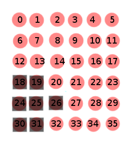
The dark squares represent obstacles.
A person can easily generate a good solution for this problem:
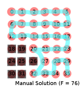
Using the GA code, we get the following:
Manual good solution ([0, 1, 2, 3, 4, 5, 11, 10, 9, 8, 7, 6, 12, 13, 14, 15, 16, 17, 23, 22, 21, 20, 21, 22, 23, 28, 27, 32, 33, 34, 28, 29, 35], ‘obstacleCount:’, 0, ‘targetCount:’, 29, ‘pathDistance:’, 34.0, ‘numTurns’, 14, ‘fitness:’, 76.0)
GA solution 1
Running the GA, we get a clearly subpar result:
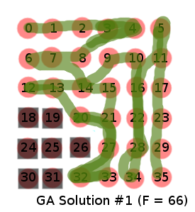
GA ‘best’ solution ([0, 1, 2, 3, 4, 3, 8, 7, 6, 7, 14, 15, 21, 27, 33, 32, 27, 21, 20, 13, 12, 13, 14, 9, 10, 16, 22, 28, 34, 28, 22, 16, 11, 5, 11, 17, 23, 29, 35], ‘obstacleCount:’, 0, ‘targetCount:’, 29, ‘pathDistance:’, 44.0, ‘numTurns’, 21, ‘fitness:’, 66.0)
Visually, we see a much worse result. This is reflected in the fitness, which is lower than our manual solution. Since GA is random, we should check with another run.
GA solution 2
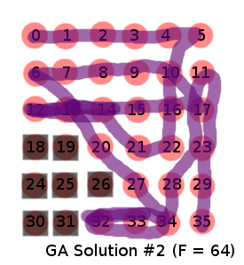
GA ‘best’ solution ([0, 1, 2, 3, 4, 5, 10, 16, 22, 21, 14, 13, 12, 13, 14, 15, 16, 17, 10, 9, 8, 7, 6, 13, 20, 27, 34, 33, 32, 33, 34, 28, 23, 17, 11, 17, 23, 29, 35], ‘obstacleCount:’, 0, ‘targetCount:’, 29, ‘pathDistance:’, 46.0, ‘numTurns’, 15, ‘fitness:’, 64.0)
Again, a poorer result with a lower fitness to match.
If we look at the rate of convergence, we get a clue as to why we cannot match the fitness of the manually-found solution.
Convergence, from GA solution 1:
  gen,nevals,avg,min,max
  0,300,-158.24,-960,36
  1,169,-48.8133,-494,38
  2,170,-18.8933,-248,42
  3,147, -5.48667,-210,42
  4,142,3.70667, -394,44
  5,164,12.8067, -212,46
  6,149,26.12,-100,48
  7,174,28.96,-202,48
  8,150,31.5533, -220,48
  9,139,37.16,-176,56
  10,149,40.3533,-164,56
  11,182,36.4267,-192,58
  12,149,41,-166,58
  13,172,35.9533,-192,60
  14,179,41.7267,-262,60
  15,156,48.6533,-156,62
  16,161,52.54,-68,66
  17,145,56.4533,-50,66
  18,178,54.56,-148,66
  19,155,55.0067,-174,66
  20,155,58.5333,-76,66
  21,136,59.9333,-58,66
  22,151,61.3667,-86,66
  23,147,61.3533,-90,66
  24,151,61.5533,-80,66
  25,145,.4067,-80,66
GA converged to a local minimum in 17 generations! Having done hundreds of GA using a variety of fitness functions, problem representations, and even using other algorithms such as particle swarm optimization and bee colony, I can say that premature convergence is very common with the coverage planning task.
Why is this? The individual chromosome is a sequence of action directives. This can be formulated as a sequence of waypoints, as in the example, or as movement actions (UP, DOWN, LEFT, etc). For any gene in the chromosome, the relative fitness of a value is extremely dependent on every other gene in the chromosome. A “good” GA formulation has values that can increase/decrease the fitness with less dependency on other genes. Consider a chromosome with two values X and Y. The fitness is some function where you maximize the result. If the Y value is bad (far from the optimal) and the X value is good (close to the optimal), the X value will increase the overall fitness. If X strays from the optimal, the fitness gets worse. So, as the fitness is modified by X and Y values, the direction to change X and Y is revealed. But in this problem, the X and Y are so tightly coupled, that the direction to modify individual good values is not clear. Typically, any random change to a decent solution only hurts the solution. A high fitness is so because of the complex interaction of every gene. In this case, 20 of them. Any change to that structure is much more likely to harm than to help. I believe this is made intuitive in the next graphic.
Crossover of GA solutions 1 and 2.
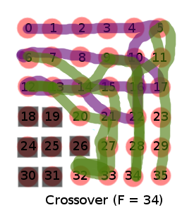
([0, 1, 2, 3, 4, 5, 10, 16, 21, 27, 22, 23, 22, 15, 14, 13, 12, 13, 14, 15, 16, 17, 10, 9, 8, 7, 6, 7, 14, 15, 21, 27, 33, 32, 27, 21, 20, 13, 12, 13, 14, 9, 10, 16, 22, 28, 27, 28, 22, 16, 11, 5, 11, 17, 23, 29, 35], ‘obstacleCount:’, 0, ‘targetCount:’, 28, ‘pathDistance:’, 66.0, ‘numTurns’, 32, ‘fitness:’, 34.0)